The Ultimate Wave Predictor

The Ultimate Wave Predictor starts with the least squares estimator. The basic formulation is the following form

where the data points, vectors and matrix are defined as:

The expression is the pseudo inverse matrix of and can be represented by in the basic formulation where,

and the basic formulation can be rewritten to the alternate form of

Observational side note, the expression is very similar to another expression, . The values in the Data Points are typically set on a regular integer interval. The example below shows an interval of 1,

The values are the sample data for each corresponding interval. As an example, we can find the linear regression of 10 data points using the formulation. Below is an n-x-y sample table of some data points.

n	x	y
0	1	0.87
1	2	10.48
2	3	24.94
3	4	39.91
4	5	45.04
5	6	56.81
6	7	56.40
7	8	74.83
8	9	75.44
9	10	88.61

The position matrix is,

The pseudo inverse matrix becomes,

and reduces to,

The data vector is,

The polynomial vector works out to,

The linear regression formulation then is the following,

The formulation can now be approximated to a decimal value of,

The approximate linear regression line is the following equation,

The plot of the data points and the linear regression is shown next.

The Ultimate Wave Predictor is derived from the least squares estimator. However, in the current process of formulation there is a problem. The process leads to an equation that is dependent on the variable. There is a way to eliminate the variable in an alternate process and have the prediction value only based on values.

The alternate process can work for any Position Matrix format of , however, we will use a special case for our Ultimate Wave Predictor. The special case is when the Position Matrix is a square matrix. The square matrix allows the pseudo inverse matrix to reduce to a simpler form. When , the matrix simplifies to and the formulation becomes .

To eliminate the variable, we need to transform the components in the data points, position matrix, and the value in the polynomial vector. The values in the data points are transformed from a fixed set value to an anywhere positional base point, , and a scalable interval differential, . Each data point increments out from the base point on an integer based value of . The basic expression representing this set is and is substituted in the data point set as follows,

This has the effect of changing the position matrix to,

When , the position matrix rewrites to,

The value in the polynomial vector is transformed to the next interval in the series of values, , and when the polynomial vector changes to,

The values are unchanged and when we go through the formulation, the and values will drop out; the value will drop, but will return in a tracking scheme that leads to a set of equations used in the final equation. The formulation then becomes,

From here we will work an expansion set of equations to see where the projections lead and will be further refined into a final equation. Starting with the zeroth degree, , we can derive the first equation.

Polynomial Vector,

Position Matrix,

Pseudo Inverse Matrix,

Data Vector,

Zeroth Degree Formulation,

This is the beginning equation in the set,

Next we will work the first degree where

Polynomial Vector,

Position Matrix,

Pseudo Inverse Matrix,

Data Vector,

First Degree Formulation,

And a one more for a third step, a second degree equation when .

Polynomial Vector,

Position Matrix,

Pseudo Inverse Matrix,

Data Vector,

Second Degree Formulation,

In each of the formulations the and values drop out and leaves only values. The drops out making it like a vector that can be positioned anywhere and drops out making it automatically scalable to any size interval; nanometers, seconds, etc. The continuation of the expansion is given in the table below out to the tenth degree. Each of the equations are the projection to just the next interval beyond the data point to for their associated polynomial regression.

n	Projection Equation
0
1
2
3
4
5
6
7
8
9
10

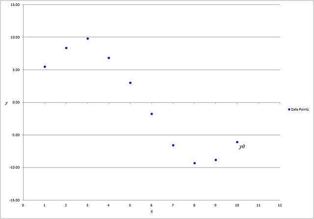
The projection equations work best for data that oscillates about the axis like a sine or cosine function. The projection equations start at the last data point and the data point moves backward from the last data point for each successive equation. The following table is an example of a sample set that oscillates about the axis and is plotted in the graph to the right.

x	y
1	5.51
2	8.39
3	9.80
4	6.84
5	3.00
6	-1.75
7	-6.58
8	-9.33
9	-8.80
10	-6.06

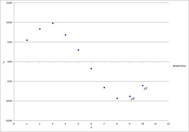
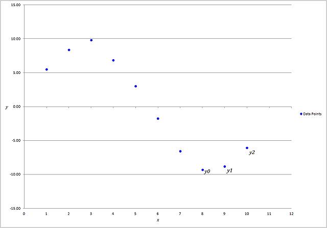
Below is shown how at each successive projection equation the data points change in relation the last point.

0^th Degree Projection,	1^st Degree Projection,
2^nd Degree Projection,	3^rd Degree Projection,

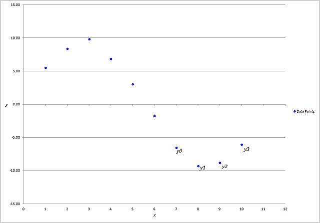
Below is a graph of 7 regression lines that project for the next possible data point at the 11^th interval; in addition, each regression equation is shown right of the legend.

The possible projections can be found using the regression equations or as we have shown earlier, using the Projection Equations. The projection equations give the same value as the regression equations for the same relative degree of the regression polynomial. There are two problems to consider at this point: first, the backward movement of the values in the projection equations needed to calculate the possible projections and second, the many possible projections as an outcome.

First we need to make the values relative to the last data point. We do this by transforming the sequence of to a sequence of to match the last data point position. Below is the table of projection equations.

n	Projection Equation
0
1
2
3
4
5
6
7
8
9
10

The starts at and moves backward at each increasing degree of the projection equation; shown in the column above. When , next when , next when , etc. Likewise, when , next when , next when , etc. We repeat the substitution for each value in the table above and the projection equations transform to the following table below.

n	Relative Projection Equation
0
1
2
3
4
5
6
7
8
9
10

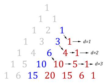
Now, we can reorder the right side of the equations, remove the column and add a column to indicate the depth of how far back in the data point set the equation is going. The value also closely relates to the familiar pattern, Pascal’s triangle, and the Binomial Formula; where . This is the 1^st level of the projection equations.

d	1^st Level Relative Projection Equation
1
2
3
4
5
6
7
8
9
10
11

Next we can find a progressive set of averages that use the many possible projections in each set by summing each equation set starting with , then , and , and so on. This will give the 2^nd level of the projection equations. The following table shows the progression.

d	Summation of Each Progressive 1^st Level Relative Projection Equation
1
2
3
4
5
6
7
8
9
10
11

This table can be reformed by grouping the like terms as follows and the coefficient summations.

d	Summation of Each Progressive 1^st Level Relative Projection Equation
1
2
3
4
5
6
7
8
9
10
11

Each summation can be reduced to the following.

d	2^nd Level Relative Projection Equation
1
2
3
4
5
6
7
8
9
10
11

The average is obtained by dividing each side of the equation by the coefficient. To find the 3^rd level, it’s best to leave the table as is, because each successive progression in levels is just the coefficient summations.

d	3^rd Level Relative Projection Equation
1
2
3
4
5
6
7
8
9
10
11

Again, to find the average, divide both sides of the equation by the coefficient.

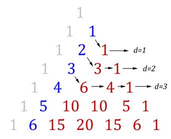
Each level, , can be associated with a different portion of the Pascal Triangle. Below are each of the 3 levels for just the first 6 depths and the associated Pascal Triangle.

d	1^st Level Relative Projection Equation
1
2
3
4
5
6

d	2^nd Level Relative Projection Equation
1
2
3
4
5
6

d	3^rd Level Relative Projection Equation
1
2
3
4
5
6

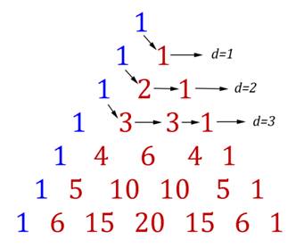
Each coefficient on the right side of the equations oscillates between + and – starting with + at . From this we can now create a single formula to express the projection for based on a depth and level for the data point observations of the values only.

If is the regular interval sample data, is the depth backward in the sample data starting at , given that and is the level of averaged projection points; with the expression as the Binomial Formula, then the Unified Equation is the following.

Solve for to get the Ultimate Wave Predictor, divide both sides by .